Survival Analysis : Part 1

Introduction

Hie there ,welcome back to one of my presentations ,This presentation will cover some basics of survival analysis, and the following series of tutorial papers can be helpful for additional reading:

further reading

Clark, T., Bradburn, M., Love, S., & Altman, D. (2003). Survival analysis part I: Basic concepts and first analyses. 232-238. ISSN 0007-0920.

M J Bradburn, T G Clark, S B Love, & D G Altman. (2003). Survival Analysis Part II: Multivariate data analysis – an introduction to concepts and methods. British Journal of Cancer, 89(3), 431-436.

Bradburn, M., Clark, T., Love, S., & Altman, D. (2003). Survival analysis Part III: Multivariate data analysis – choosing a model and assessing its adequacy and fit. 89(4), 605-11.

Clark, T., Bradburn, M., Love, S., & Altman, D. (2003). Survival analysis part IV: Further concepts and methods in survival analysis. 781-786. ISSN 0007-0920.

# setup

In this section, we will use the following packages:

library(survival)
library(survminer)
library(lubridate)
library(ggsurvfit)
library(gtsummary)
library(tidyverse)

## basic Definitions in survival analysis

• Survival analysis lets you analyze the rates of occurrence of events over time, without assuming the rates are constant.
• Generally, survival analysis lets you model the time until an event occurs,
• In the medical world, we typically think of survival analysis literally ,tracking time until death. But, it’s more general than that
• survival analysis models time until an event occurs (any event).
• This might be death of a biological organism.
• But it could also be the time until a hardware failure in a mechanical system,
• time until recovery,
• time someone remains unemployed after losing a job,
• time until a ripe tomato is eaten by a grazing deer,
• time until someone falls asleep in a workshop, etc.
• Survival analysis also goes by reliability theory in engineering,
• duration analysis in economics, and event history analysis in sociology.

Special features of survival data😝

• Survival times are generally not symmetrically distributed. - Usually the data is positively skewed and it will be unreasonable to assume that of this type have a normal distribution. However data can be transformed to give a more symmetric distribution. - Survival times are frequently censored. The survival time of an individual is said to be censored when the end-point of interest has not been observed for that individual.

Example of the distribution of follow-up times according to event status:

library(paletteer)
ggplot(lung, aes(x = time, fill = factor(status))) +
  geom_histogram(bins = 25, alpha = 0.5, position = "identity") +
  scale_fill_manual(values = paletteer_c("ggthemes::Blue", 3), 
                    labels = c("Censored", "Dead")) +
  
  labs(x = "Days",
       y = "Count")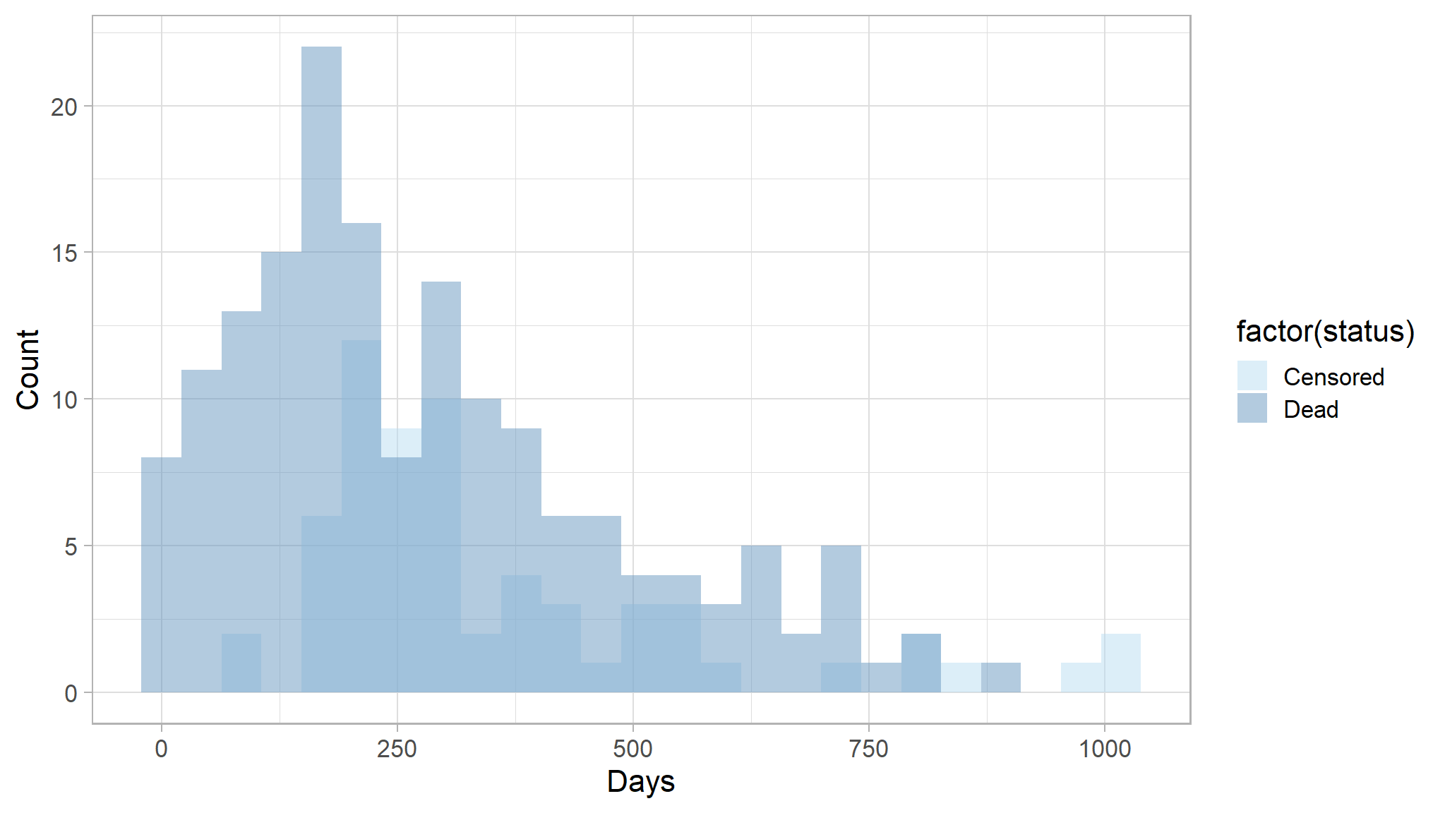

censoring

• Censoring is a type of missing data problem unique to survival analysis. - This happens when you track the sample/subject through the end of the study and the event never occurs. - This could also happen due to the sample/subject dropping out of the study for reasons other than death, or some other loss to followup. The sample is censored in that you only know that the individual survived up to the loss to followup, but you don’t know anything about survival after that.

A subject may be censored due to:

• Loss to follow-up

• Withdrawal from study

- No event by end of fixed study period

Specifically these are examples of right censoring.

• Left censoring and interval censoring are also possible, and methods exist to analyze these types of data, but this tutorial will be focus on right censoring.

illustrating the impact of censoring:

# make fake data
fkdt <- tibble(Subject = as.factor(1:10), 
              Years = sample(4:20, 10, replace = T),
              censor = sample(c("Censor", rep("Event", 2)), 10, 
              replace = T)) 

# plot with shapes to indicate censoring or event
ggplot(fkdt, aes(Subject, Years)) + 
    geom_bar(stat = "identity", width = 0.5) + 
    geom_point(data = fkdt, 
               aes(Subject, Years, 
                   color = censor, shape = censor), 
               size = 6) +
    coord_flip() +
    theme_minimal() + 
    theme(legend.title = element_blank(),
          legend.position = "bottom")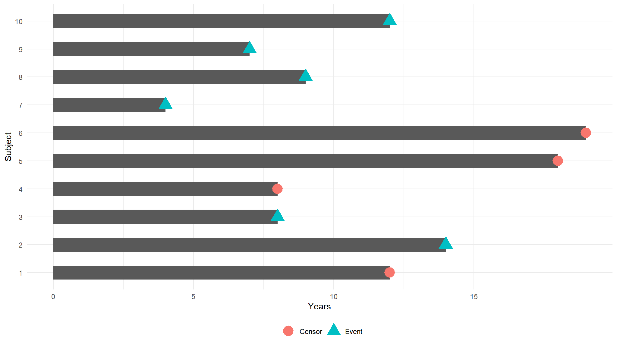

whats happening

• Subjects 6 and 7 were event-free at 10 years.

• Subjects 2, 9, and 10 had the event before 10 years.

- Subjects 1, 3, 4, 5, and 8 were censored before 10 years, so we don’t know whether they had the event or not at 10 years. But we know something about them

- that they were each followed for a certain amount of time without the event of interest prior to being censored.

types of censoring

• If the individual was last known to be alive at time \(t_0 + C\), the time c is called a censored survival time. This censoring occurs after the individual has been entered into a study, that is, to the right of the last known survival time, and is therefore known as right censoring. The right-censored survival time is then less than the actual, but unknown, survival time.

• which is encountered when the actual survival time of an individual is less than that observed. To illustrate this form of censoring, consider a study in which interest centres on the time to recurrence of a particular cancer following surgical removal of the primary tumour. Three months after their operation, the patients are examined to determine if the cancer has recurred. At this time, some of the patients may be found to have a recurrence. For such patients, the actual time to recurrence is less than three months,

Survivor and hazard functions

• The hazard is the instantaneous event (death) rate at a particular time point t. Survival analysis doesn’t assume the hazard is constant over time. The cumulative hazard is the total hazard experienced up to time t.

• The survival function, is the probability an individual survives (or, the probability that the event of interest does not occur) up to and including time t. It’s the probability that the event (e.g., death) hasn’t occured yet. It looks like this, where \(T\) is the time of death, and \(Pr(T>t)\) is the probability that the time of death is greater than some time \(t\). \(S\) is a probability, so \(0 \leq S(t) \leq 1\), since survival times are always positive (\(T \geq 0\)). > probability that an individual survives beyond any given time

\[ S(t) = Pr(T>t) \]

Survival function

Survival analysis typically involves using T as the response variable, as it represents the time till an outcome occurs, while t refers to the actual survival time of an individual. The distribution function F(t) is used to describe chances of time of survival being less than a given value, t. In some cases, the cumulative distribution function is of interest and can be obtained as follows:

\[F(t)=P(T\le t)=\int_{t}^{\infty}f(u)\]

• Interest also tends to focus on the survival or survivorship function which in a study is the chances of a neonate surviving after time \(t\) and also given by the formula

\(S(t)\) monotonically decreasing function with \(S(0) = 1\) and \(S(\infty) = \text{lim}_{t \rightarrow \infty} S(t) = 0\).

Hazard function

Suppose we have \(R (t)\) (set at risk) that has neonates who are prone to dying by time t, the chances of a neonate in that set to die in a given interval \([t, t + \delta t)\) is given by the following forrmula, where \(h(t)\) is the hazard rate and is defined as:

\[h(t) = \lim_{\delta t \rightarrow 0} \frac{P(t \le T < t+\delta t | T \ge t)}{\delta t}\] The hazard function’s shape can be any strictly positive function and it changes based on the specific survival data provided.

Relationship between h(t) and S(t)

we know that \(f(t) = - \frac{d}{dt} S(t)\) hence equation simplifies to

\[h(t)=\frac{f(t)}{S(t)} =\frac{- \frac{d}{dt} S(t)}{S(t)}= - \frac{d}{dt} [\log S(t)]\]

Taking intergrals both sides the above reduces to: \[H(t)= -\log S(t)\]

where \(H(t)=\int_{t}^{t} h(u) du\) ,is the cumulative risk of a neonate dying by time t. Since the event is death, then H(t) summarises the risk of death up to time t, assuming that death has not occurred before t. The survival function is also approximately simplified as follows. \[ S(t) = e^{-H(t)} \approx 1 -H(t) \text{ when H(t) is small. }\]

Kaplan-Meier estimate

If there are \(r\) times of deaths among neonates in ICU, such that \(r\leq n\) and \(n\) is the number of neonates with observed survival times. Arranging these times in from the smallest to the largest,the \(j\)-th death time is noted by \(t_{(j)}\) , for \(j = 1, 2, \cdots , r\), such that the \(r\) death times ordred are \[ t_{1}<t_{2}< \cdots < t_{m}\] .

Let \(n_j\), for \(j = 1, 2, \ldots, r\), denote the number of neonates who are still alive before time \(t(j)\), including the ones that are expected to die at that time. Additionally, let \(d_j\) denote the number of neonates who die at time \(t(j)\). The estimate for the product limit can be expressed in the following form:

\[\hat{S}(t) = \prod_{j=1}^k \, \left(1-\frac{d_j}{r_j}\right)\]

To survive until time \(t\), a neonate must start by surviving till \(t(1)\), and then continue to survive until each subsequent time point \(t(2), \ldots, t(r)\). It is assumed that there are no deaths between two consecutive time points \(t(j-1)\) and \(t(j)\). The conditional probability of surviving at time \(t(i)\), given that the neonate has managed to survive up to \(t(i-1)\), is the complement of the proportion of the new born babies who die at time \(t(i)\), denoted by \(d_i\), to the new born babies who are alive just before \(t(i)\), denoted by \(n_i\). Therefore, the probability that is conditional of surviving at time \(t(i)\) is given by \(1 - \frac{d_i}{n_i}\).

The variance of the estimator is given by \[\text{var}(\hat{S}(t)) = [\hat{S}(t)]^2 \sum_{j=1}^k \frac{d_j}{(r_j-d_j) r_j}\]

The corresponding standard deviation is therefore given by: \[\text{s.e}(\hat{S}(t)) = [\hat{S}(t)]\left[\sum_{j=1}^k \frac{d_j}{(r_j-d_j) r_j}\right]^{\frac{1}{2}}\]

The Kaplan-Meier curve illustrates the survival function. It’s a step function illustrating the cumulative survival probability over time. The curve is horizontal over periods where no event occurs, then drops vertically corresponding to a change in the survival function at each time an event occurs.

Log rank test

Given the problem of contrasting two or more survival functions,for instance survival times between male and female neonates in the ICU. Let \[ t_{1}<t_{2}< \cdots < t_{r}\]

Let \(t_i\) be the unique times of death observed among the neonates, found by joining all groups of interest. For group \(j\),\ let \(d_{ij}\) denote the number of deaths at time \(t_i\), and\ let \(n_{ij}\) denote the number at risk at time \(t_i\) in that group. Let \(d_i\) denote the total number of deaths at time \(t_i\) across all groups, and\

the expected number of deaths in group \(j\) at time \(t_i\) is: ,

\[E(d_{ij}) = \frac{n_{ij} \, d_i}{n_i} = n_{ij} \left(\frac{d_i}{n_i}\right) \]

At time \(t_i\), suppose there are \(d_i\) deaths and \(n_i\) individuals at risk in total, with \(d_{i0}\) and \(d_{i1}\) deaths and \(n_{i0}\) and \(n_{i1}\) individuals at risk in groups 0 and 1, respectively, such that \(d_{i0} + d_{i1} = d_i\) and \(n_{i0} + n_{i1} = n_i\). Such data can be summarized in a \(2 \times 2\) table at each death time \(t_i\).

Given that the null hypothesis is true, the number of deaths is expected to follow the hypergeometric distribution, and therefore: \[E(d_{i0}) =e_{i0}= \frac{n_{i0} \, d_i}{n_i} = n_{i0} \left(\frac{d_i}{n_i}\right)\]

\[\text{Var}(d_{i0}) = \frac{n_{i0} \, n_{i1} \, d_i(n_i-d_i)}{n_{i}^2 (n_{i}-1)}\]

the statistic \(U_L\) is given by \[U_L=\sum^r_{i=1}(d_{i0}-e_{i0})\] so that the variance of \(U_L\) is \[Var(U_L)=\sum^r_{j=1}v_{i0}=V_L\] which then follows that : \[\frac{U_L}{\sqrt{V_L}} \sim N(0,1)\] and squaring results in \[\frac{U^2_L}{V_L}\sim \chi^2_1\]

Regression models in Survival analysis

Cox’s Proportional Hazards

The model is semi-parametric in nature since no assumption about a probabilty distribution is made for the survival times. The baseline model can take any form and the covariate enter the model linearly (Fox,2008). The model can thus be represented as :

\[h(t|X) = h_0(t) \exp(\beta_1 X_{1} + \cdots + \beta_p X_{p})=h_0(t)\text{exp}^{(\beta^{T} X)}\]

In the above equation, \(h_0(t)\) is known as the baseline hazard function, which represents the hazard function for a neonate when all the included variables in the model are zero. On the other hand, \(h(t|X)\) represents the hazard of a neonate at time \(t\) with a covariate vector \(X=(x_1,x_2,\ldots,x_p)\) and \(\beta^T=(\beta_1,\beta_2,\ldots,\beta_p)\) is a vector of regression coefficients.

Fitting a proportional hazards model

The partial likelihood

Given that \(t(1) < t(2) < \ldots < t(r)\) denote the \(r\) ordered death times. The partial likelihood is given by :

\[L(\beta) = \prod_{i=1}^{n} \left[\frac{\text{exp}^{\beta ^{T} X_i}}{ \sum_{\ell\in R(t_{(i)}}\text{exp}^{\beta ^{T} X_\ell}}\right]^{\delta_i}\]

Maximising the logarithmic of the likelihood function is more easier and computationally efficient and this is generally given by:

\[\log L(\beta)= \sum_{i=1}^{n} \delta_i \left[ \beta ^{T} X_i - \log \left(\sum_{\ell \in R(t_{(i)}}\text{exp}^{\beta ^{T} X_\ell}\right) \right]\]

Residuals for Cox Regression Model

Six types of residuals are studied in this thesis: Cox-Snell, Modified Cox-Snell, Schoenfeld, Martingale, Deviance, and Score residuals.

Cox-Snell Residuals

Cox-Snell definition of residuals given by Cox and Snell (1968) is the most common residual in survival analysis. The Cox-Snell residual for the \(ith\) individual, \(i = 1, 2, \cdots , n\), is given by

\[r_{Ci}=\text{exp}(\mathbf{\hat{\beta}^{T} x_i})\hat{H}_0(t_i)\]

where \(\hat{H}_0(t_i)\) is an estimate of the baseline cumulative hazard function at time \(t_i\). It is sometimes called the Nelson-Aalen estimator.

Martingale residuals

These are useful in determing the functional form of the covariates to be included in the model. If the test reveals that the covariate can not be included linearly then there is need for such a covariate to be transformed . The martingale residuals are represented in the following form

\[r_{Mi}=\delta_i - r_{Ci}\]

Deviance Residuals

The skew range of Martingale residual makes it difficult to use it to detect outliers. The deviance residuals are much more symmetrically distributed about zero and are defined by

\[r_{Di}=\text{sgn}(r_{Mi})\left[-2\{r_{Mi}+\delta_i\log\left(\delta_i-r_{Mi}\right)\}\right]^{\frac{1}{2}}\]

Here, \(r_{Mi}\) represents the martingale residual for the \(i\)-th individual, and the function \(\text{sgn}(\cdot)\) denotes the sign function. Specifically, the function takes the value +1 if its argument is positive and -1 if negative.

Schoenfield residuals

Schoenfeld residuals are a useful tool for examining and testing the proportional hazard assumption, detecting leverage points, and identifying outliers. They can be calculated as follows:

\[r_{Sji}=\delta_i\{x_{ji}-\hat{a}_{ji}\}\]

where \(x_{ji}\) is the value of the \(jth\) explanatory variable,\(j = 1, 2, \cdots , p\), for the \(ith\) individual in the study,

\[\hat{a}_{ji}=\frac{\sum_{\ell \in R(t_i)}x_{j\ell}\text{exp}(\mathbf{\hat{\beta}^{T} x_{\ell}})}{\sum_{\ell \in R(t_i)}\text{exp}(\mathbf{\hat{\beta}^{T} x_{\ell}})}\]